如题，笔者作为队伍中的编程手，将在此分享自己的准备历程。队伍准备打MothorCup和电工杯，最终在9月份参加国赛。

3.15

线性规划模型:

from scipy import optimize
import numpy as np

c = np.array([-4,-3]) # 默认求最小值 所以求最大值时需要加 - 
A = np.array([[2,1],[1,1],[0,1]]) #默认求Ax<=b 需要加-如果是>=
b = np.array([10,8,7])
A_eq = np.array([])#没有等式
b_eq = np.array([])

res = optimize.linprog(c,A,b)
print(res)

https://www.cnblogs.com/youcans/p/14713335.html
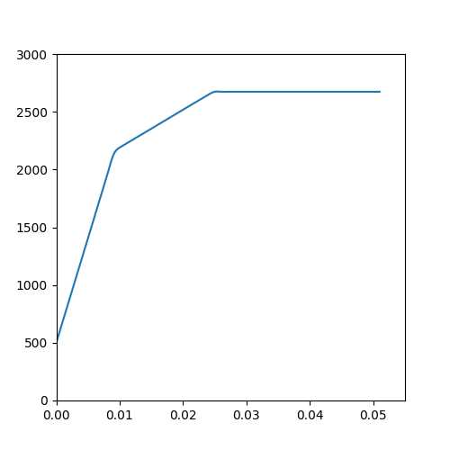
练习 & matplotlib 平滑曲线，标记x,y轴

from scipy import optimize
import numpy as np
import matplotlib.pyplot as plt 
from scipy.interpolate import make_interp_spline

a = 0
a_list = []
res_list = []
while a<0.05:
    M = 10000
    c = np.array([-0.05,-0.27,-0.19,0.185,0.185]) # 默认求最小值 所以求最大值时需要加 - 
    A = np.array([[0.0,0,0,0,0],[0,0.025,0,0,0],[0,0,0.015,0,0],[0,0,0,0.055,0],[0,0,0,0,0.026]]) #默认求Ax<=b 需要加-如果是>=
    b = np.array([a*M,a*M,a*M,a*M,a*M])
    A_eq = np.array([[1.0,1.01,1.02,1.045,1.065]])
    b_eq = np.array([M])
    res = optimize.linprog(c,A,b,A_eq,b_eq)
    a_list.append(a)
    res_list.append(-res.fun)
    a+=0.001
fig = plt.figure(num=1, figsize = (5,5))
ax = fig.add_subplot(1,1,1)
model = make_interp_spline(a_list, res_list)
xs = np.linspace(0,0.051,1000)
ys = model(xs)
ax.plot(xs,ys)
ax.set_xlim(0,0.055)
ax.set_ylim(0,3000)
#ax.set_xticks(np.linspace(1,10,10))
ax.set_yticks(np.linspace(0,3000,7))
plt.savefig('figure.jpg')
plt.show()

成果:

3.17

整数规划模型：
先去除整数的约束，得到松弛解
如果所有变量均为整数，则返回
如果不为整数，如x0为c
则分别添加x0<=floor(c)和x0>=ceil(c)递归运算两次
或者使用pulp 库

import pulp as pp
c = [1,1,1,1,1,1]
A_gq = [[1,0,0,0,0,1],[1,1,0,0,0,0],[0,1,1,0,0,0],[0,0,1,1,0,0],[0,0,0,1,1,0],[0,0,0,0,1,1]]
b_gq = [35,40,50,45,55,30]

m = pp.LpProblem(sense=pp.LpMinimize)
x = [pp.LpVariable(f'x{i}',lowBound=0,cat='integer') for i in range(1,7)]
m += pp.lpDot(c,x)
for i in range(len(A_gq)):
    m += (pp.lpDot(A_gq[i],x)>=b_gq[i])
m.solve()
print(f'优化结果：{pp.value(m.objective)}')
print(f'参数取值：{[pp.value(var) for var in x]}')

非线性规划：

from scipy import optimize
import numpy as np

func = lambda x: (2+x[0])/(1+x[1])-3*x[0]+4*x[2]
cons = (
{'type':'ineq', 'fun': lambda x: x[0]-0.1},
{'type':'ineq', 'fun': lambda x: -x[0]+0.9},
{'type':'ineq', 'fun': lambda x: x[1]-0.1},
{'type':'ineq', 'fun': lambda x: -x[1]+0.9},
{'type':'ineq', 'fun': lambda x: x[2]-0.1},
{'type':'ineq', 'fun': lambda x: -x[2]+0.9}
)
x0 = np.asarray((0.5,0.5,0.5,0.5))
res = optimize.minimize(func,x0,method='SLSQP',constraints=cons)
print(res.fun)
print(res.success)
print(res.x)

# 求x0附近的局部最优解 ineq是大于等于0

3.18

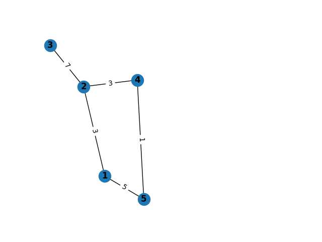
图论的可视化

import networkx as nx
import matplotlib.pyplot as plt
G = nx.Graph()
G.add_node(1)
G.add_node(2)
G.add_nodes_from([3,4])
G.add_node(5,color='white')
G.add_weighted_edges_from([(1,2,3)])
G.add_weighted_edges_from([(3,2,7),(4,5,1),(5,1,5),(4,2,3)])

pos = nx.spring_layout(G)
labels = nx.get_edge_attributes(G,'weight')

subax1 = plt.subplot(121)
nx.draw(G,pos,with_labels=True, font_weight='bold')
nx.draw_networkx_edge_labels(G, pos ,edge_labels = labels)
plt.show()

3.21

一点最大流： https://www.cnblogs.com/SYCstudio/p/7260613.html

3.25

多项式拟合：

import numpy as np
import matplotlib.pyplot as plt

x = np.linspace(10,80,8)
y = np.array([174,236,305,334,349,351,342,323])

f1 = np.polyfit(x,y,3) #3 stands for the highest degrees
p1 = np.poly1d(f1)
print('p1 is :n',p1)
plt.plot(x,y,'s',label='original values')
yvals = p1(x)
plt.plot(x,yvals,'r',label='polyfit values')
plt.show()

自定义函数拟合(func)可以自行修改：

import numpy as np
import matplotlib.pyplot as plt
from scipy.optimize import curve_fit

x = np.linspace(10,80,8)
y = np.array([174,236,305,334,349,351,342,323])

def func(x,a,b,c):
    return a*np.sqrt(x)*(b*np.square(x)+c)

popt, pcov = curve_fit(func,x,y)
yvals = func(x,*popt)
plt.plot(x,y,'s',label='original values')
plt.plot(x,yvals,'r',label='polyfit values')
plt.show()

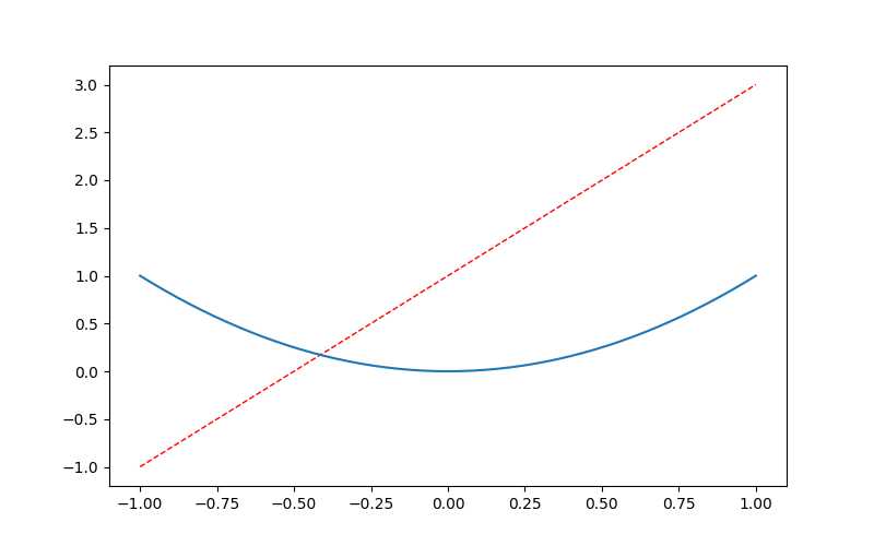
matplot初探 指路：莫烦

import matplotlib.pyplot as plt
import numpy as np

x = np.linspace(-1,1,51)
y1 = 2*x+1
y2 = x**2
plt.figure(figsize=(8,5))
plt.plot(x,y1,color='red',linewidth=1.0,linestyle='--')
plt.plot(x,y2)
plt.show()

4.6

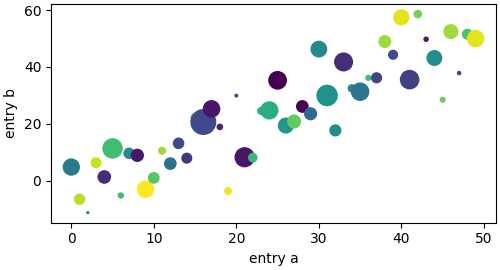
matplotlib 散点图：

import numpy as np
import matplotlib.pyplot as plt
np.random.seed(19680801)  # seed the random number generator.
data = {'a': np.arange(50),
        'c': np.random.randint(0, 50, 50),
        'd': np.random.randn(50)}
data['b'] = data['a'] + 10 * np.random.randn(50)
data['d'] = np.abs(data['d']) * 100

fig, ax = plt.subplots(figsize=(5, 2.7), layout='constrained')
ax.scatter('a', 'b', c='c', s='d', data=data) # c: color s: size
ax.set_xlabel('entry a')
ax.set_ylabel('entry b')
plt.show()

多数据图像：

import numpy as np
import matplotlib.pyplot as plt

x = np.linspace(0,2,100)
fig,ax  = plt.subplots(figsize=(5,2.7),layout='constrained')
ax.plot(x, x, label='linear')
ax.plot(x, x**2, label='quadratic')
ax.plot(x, x**3, label='cubic')
ax.set_xlabel('x label')
ax.set_ylabel('y label')
ax.set_title('Simple Plot')
ax.legend()
plt.show()

matplotlib 颜色：
https://matplotlib.org/stable/users/explain/colors/colors.html#colors-def]

matplotlib 加文本:
ax.text(x, y, s) 其中x y为值坐标 例如x为[1,100] 50 在中间

4.8

模拟退火算法
设定初始温度，想求解函数为能量E；每次变成新低温状态的概率为e^{\frac{-\Delta E(i)}{T}}.
链接：https://oi-wiki.org/misc/simulated-annealing/

```C++
// https://www.luogu.com.cn/problem/P1337
using namespace std;

typedef long long ll;
typedef pair<int,int> pii;

const int maxn=1005;
const int INF=1e9+7;

int read(){
int x=0,f=1,c=getchar();
while(c<'0'||c>'9'){if(c<span class="text-highlighted-inline" style="background-color: #fffd38;">'-')f=-1;c=getchar();}
while(c>='0'&&c<='9'){x=x<em>10+(c-'0');c=getchar();}
return x</em>f;
}</span>

double Rand(){return (double)rand()/RAND_MAX;}

int n;
int x[maxn],y[maxn],w[maxn];
double ansx,ansy,dis;

double calc(double nowx,double nowy){
double nowdis = 0;
for(int i=0;i<n;++i){
double dx = nowx-x[i], dy = nowy-y[i];
nowdis += sqrt(dx<em>dx+dy</em>dy) * w[i];
}
if(nowdis < dis){ansx=nowx;ansy=nowy;dis=nowdis;}
return nowdis;
}

void SimulateAnneal(){
double T = 1000000;
double nowx = ansx, nowy = ansy;
double D = calc(nowx,nowy);
while(T>0.001){
double newx = nowx + T/10<em>(Rand()</em>2 - 1), newy = nowy + T/10<em>(Rand()</em>2-1);
double nowD = calc(newx,newy),delta = nowD-D;
if(exp(-delta/T<em>10) > Rand()) nowx=newx, nowy=newy;
T</em>=0.97;
D = nowD;
}
for(int i=0;i<1000;++i){
double nxtx = ansx+T<em>(Rand()</em>2-1), nxty = ansy+T<em>(Rand()</em>2-1);
calc(nxtx,nxty);
}
}

int main(){
srand((unsigned int)time(NULL));
n=read();
for(int i=0;i<n;++i){
x[i]=read();
y[i]=read();
w[i]=read();
ansx+=x[i];
ansy+=y[i];
}
ansx /= n;
ansy/=n;
dis = calc(ansx,ansy);
SimulateAnneal();
printf("%.3lf %.3lf\n",ansx,ansy);
return 0;
}

```